brat

The class we use to format rational functions is brat, and the kinds of rational functions accepted satisfy the main assumption: they can be expressed as [ \dfrac{F(\bm{X})}{c\bm{X}^{\beta} \prod_{i=1}^m(1 - \bm{X}^{\alpha_i})}, ]

where the following hold:

$\bm{X}=(X_1, \dots, X_n)$ are variables,
$F(\bm{X})\in \mathbb{Z}[\bm{X}]$,
$c\in \N$,
$\beta\in\N_0^n$,
$m\in\N_0$,
$\alpha_i\in\mathbb{Z}^n$, where $\bm{X}^{\alpha_i} = X_1^{\alpha_{i,1}}\cdots X_n^{\alpha_{i,n}}$.

This includes all elements of $\mathbb{Q}[\bm{X}^{\pm 1}]$ for example.

We aim to provide lots of customization with how rational functions are formatted. This can be achieved by the following keyword arguments:

rational_expression: the rational function (default: None),
numerator: the numerator polynomial of the rational function (default: None),
denominator: the denominator polynomial of the rational function (default: None),
denominator_signature: the dictionary of data for the denominator (default: None),
fix_denominator: whether to keep the given denominator fixed---does not apply to coefficients (default: True),
increasing_order: whether to display polynomials in increasing degree (default: True),
hide_monomial: whether to absorb the monomial in the denominator into the numerator (default: True),
variables: the variables, or their names, in the order to use (default: None).

Every brat with a zero numerator is 0. A brat is accepted as input to brat; given on its own it keeps the denominator it was built with, so br.brat(F) does not reshape the original F. The numerator may be a Laurent polynomial: its monomial is moved to the denominator, where the signature records it.

Denominator signature

The denominator_signature must be a dictionary with all three of the following keys—a missing or unexpected key raises an error:

"coefficient": an integer,
"monomial": a tuple of non-negative integers with length matching the number of variables,
"factors": a dictionary whose keys are tuples of integers with values of positive integers.

The dictionary you provide is never modified: brat works on a copy of it, so the same signature can be reused for several brats. Examples of acceptable denominator_signature are given in the Providing a signature example and in the denominator_signature method.

Order of the variables

The variables are kept in the order they were given in. A polynomial ring records that order, so it is the one you declared:

sage: q, t = polygens(QQ, 'q,t')
sage: br.brat((1 + q)/(1 - q*t)).variables()
(q, t)

A symbolic expression has no such order to preserve. The Symbolic Ring reports its variables alphabetically. Use variables to say what the order should be. It takes the variables themselves or their names, and the order carries through the operations:

sage: Y, T = var('Y T')
sage: br.brat((1 + Y)/(1 - Y*T), variables=(Y, T)).variables()
(Y, T)
sage: br.brat((1 + Y)/(1 - Y*T), variables=('Y', 'T')).variables()
(Y, T)

Variables that do not occur in the expression are allowed. A variable that occurs but is missing from variables raises an error.

The order is used to break ties when displaying a brat. Terms of the numerator are shown by degree, and terms of the same degree appear in the order of the variables. The factors of the denominator are shown the same way:

sage: q, t, u = polygens(QQ, 'q,t,u')
sage: br.brat(1 + q + t + u)
1 + q + t + u
sage: br.brat(1/((1 - q)*(1 - t)*(1 - u)))
1/((1 - q)*(1 - t)*(1 - u))

Algebraic operations and relations

One can use the usual algebraic operations with brat: add, subtract, multiply, divide (i.e. 'true' divide), powers. The Boolean relations == and != can also be used. When adding a brat with something else, we attempt to make another brat object.

The order of the variables of the left brat is used whenever orders differ. Variables the right operand brings with it follow, in its order:

sage: q = polygens(QQ, 'q')[0]
sage: u, x, Q = polygens(QQ, 'u,x,q')
sage: F = br.brat(1/(1 - q))
sage: G = br.brat(1/((1 - u)*(1 - x)*(1 - Q)))
sage: (F + G).variables()
(q, u, x)
sage: (G + F).variables()
(u, x, q)

A brat is hashable, so it can be used in a set or as a dictionary key. Two brats that are equal if and only if they have the same hash, and a brat has the same hash as its underlying rational function.

Warning: we cannot do anything about algebraic operations where the first object is not a brat object. For example, if F is a brat but G is a polynomial in SageMath, then G + F may raise errors, while F + G will attempt to add the two objects—other errors may arise.

Examples

We build many examples using the brat constructor.

Introduction

We express the rational function [ f=\dfrac{1 + xy + x^2y^2}{(1 - x)(1 - y)}. ] First we write this in the usual way, using symbolic variables.

sage: x, y = var('x y')
sage: f = (1 + x*y + x^2*y^2)/((1 - x)*(1 - y))
sage: f
(x^2*y^2 + x*y + 1)/((x - 1)*(y - 1))

Now we build a brat from $f$.

sage: F = br.brat(f)
sage: F
(1 + x*y + x^2*y^2)/((1 - x)*(1 - y))

Prescribed Denominator I

Now we write the rational function [ g = \dfrac{1 + 4t + 6t^2 + 4t^3 + t^4}{(1 - t)(1 - t^2)(1 - t^3)(1 - t^4)} . ]

sage: t = polygens(QQ, 't')[0]
sage: g = (1 + 4*t + 6*t^2 + 4*t^3 + t^4)/((1 - t)*(1 - t^2)*(1 - t^3)*(1 - t^4))
sage: g
(t^2 + 2*t + 1)/(t^8 - 3*t^7 + 4*t^6 - 5*t^5 + 6*t^4 - 5*t^3 + 4*t^2 - 3*t + 1)

Now we build a brat.

sage: G = br.brat(g)
sage: G
(1 + 2*t - 2*t^3 - t^4)/((1 - t)^3*(1 - t^3)*(1 - t^4))

We could instead insist that the denominator $(1 - t)(1 - t^2)(1 - t^3)(1 - t^4)$ stay fixed.

sage: G = br.brat(
    numerator=1 + 4*t + 6*t^2 + 4*t^3 + t^4,
    denominator=(1 - t)*(1 - t^2)*(1 - t^3)*(1 - t^4)
)
sage: G
(1 + 4*t + 6*t^2 + 4*t^3 + t^4)/((1 - t)*(1 - t^2)*(1 - t^3)*(1 - t^4))

By default, fix_denominator is set to True. Setting this to False yields the following.

sage: br.brat(
    numerator=1 + 4*t + 6*t^2 + 4*t^3 + t^4,
    denominator=(1 - t)*(1 - t^2)*(1 - t^3)*(1 - t^4),
    fix_denominator=False
)
(1 + 2*t - 2*t^3 - t^4)/((1 - t)^3*(1 - t^3)*(1 - t^4))

Prescribed denominator II

We construct the following rational function a few different ways: [ P = \dfrac{1 + 6T + 11T^2 + 6T^3}{(1 - T^4)}. ]

sage: T = polygens(QQ, 'T')[0]
sage: P = br.brat((1 + 6*T + 11*T^2 + 6*T^3)/(1 - T^4))
sage: P
(1 + 5*T + 5*T^2 - 5*T^3 - 6*T^4)/((1 - T)*(1 - T^4))

By doing the above construction, we added a factor of $1-T$. This is because SageMath automatically removes common factors in the numerator and denominator of the quotient (1 + 6*T + 11*T^2 + 6*T^3)/(1 - T^4). The resulting denominator is $(T - 1)(T^2 + 1)$.

sage: P = br.brat(
    numerator=1 + 6*T + 11*T^2 + 6*T^3,
    denominator=(1 - T)^4
)
sage: P
(1 + 6*T + 11*T^2 + 6*T^3)/(1 - T)^4

By separating the denominator (and fixing it by default), we get the desired expression.

We can also switch the order of how polynomials are displayed. Instead of displaying the terms in a weakly increasing-degree sequence, we can make it weakly decreasing.

sage: P = br.brat(
    numerator=1 + 6*T + 11*T^2 + 6*T^3,
    denominator=(1 - T)^4,
    increasing_order=False
)
sage: P
(6*T^3 + 11*T^2 + 6*T + 1)/(1 - T)^4

Providing a signature

We construct the following rational function using a denominator signature: [ h = \dfrac{1}{8(1 - X_1)(1 - X_2)^3(1 - X_1X_2X_3)^4(1 - X_1X_2X_3^2)}. ]

sage: R = PolynomialRing(QQ, 'X1,X2,X3')
sage: d_sig = {
    "coefficient": 8,
    "monomial": (0, 0, 0),
    "factors": {
        (1, 0, 0): 1, 
        (0, 1, 0): 3,
        (1, 1, 1): 4,
        (1, 1, 2): 1
    }
}
sage: H = br.brat(numerator=R(1), denominator_signature=d_sig)
sage: H
1/(8*(1 - X1)*(1 - X2)^3*(1 - X1*X2*X3)^4*(1 - X1*X2*X3^2))

Negative Exponents I

We express the Igusa zeta function associated with the braid arrangement: [ Z_2 = \dfrac{1 - 3q^{-1} + 2q^{-2} + 2q^{-1}t - 3q^{-2}t + q^{-3}t}{(1 - q^{-1}t)(1 - q^{-2}t^3)} . ]

See Maglione–Voll for details.

sage: q, t = var('q t')
sage: Z2 = (1 - 3*q^-1 + 2*q^-2 + 2*q^-1*t - 3*q^-2*t + q^-3*t)/((1 - q^-1*t)*(1 - q^-2*t^3))
sage: Z2
(2*t/q - 3/q - 3*t/q^2 + 2/q^2 + t/q^3 + 1)/((t^3/q^2 - 1)*(t/q - 1))
sage: br.brat(Z2)
(2*q^-2 + q^-3*t - 3*q^-1 - 3*q^-2*t + 1 + 2*q^-1*t)/((1 - q^-1*t)*(1 - q^-2*t^3))

To get the output a little closer to how we have it formatted above, we can set increasing_order to False.

sage: br.brat(Z2, increasing_order=False)
(1 + 2*q^-1*t - 3*q^-1 - 3*q^-2*t + 2*q^-2 + q^-3*t)/((1 - q^-1*t)*(1 - q^-2*t^3))

Negative Exponents II

We express the ask zeta function associated with the complete graph on four vertices: [ W_{minus} = \dfrac{q^3 - t}{q^3(1 - t)(1 - qt)}. ]

See Rossmann–Voll for details.

sage: q, t = var('q t')
sage: W_minus = (q^3 - t)/(q^3*(1 - t)*(1 - q*t))
sage: W_minus
(q^3 - t)/((q*t - 1)*q^3*(t - 1))
sage: br.brat(W_minus)
-(q^-3*t - 1)/((1 - t)*(1 - q*t))

If we set increasing_order to False, then the 1 will be the leading term, and since it has a positive coefficient, we will avoid the negative scalar in front.

sage: br.brat(W_minus, increasing_order=False)
(1 - q^-3*t)/((1 - t)*(1 - q*t))

Moreover, if we want to make the factor $q^3$ in the denominator explicit, we can set hide_monomial to False.

sage: br.brat(W_minus, increasing_order=False, hide_monomial=False)
(q^3 - t)/(q^3*(1 - t)*(1 - q*t))

Pretty Print (pretty_print)

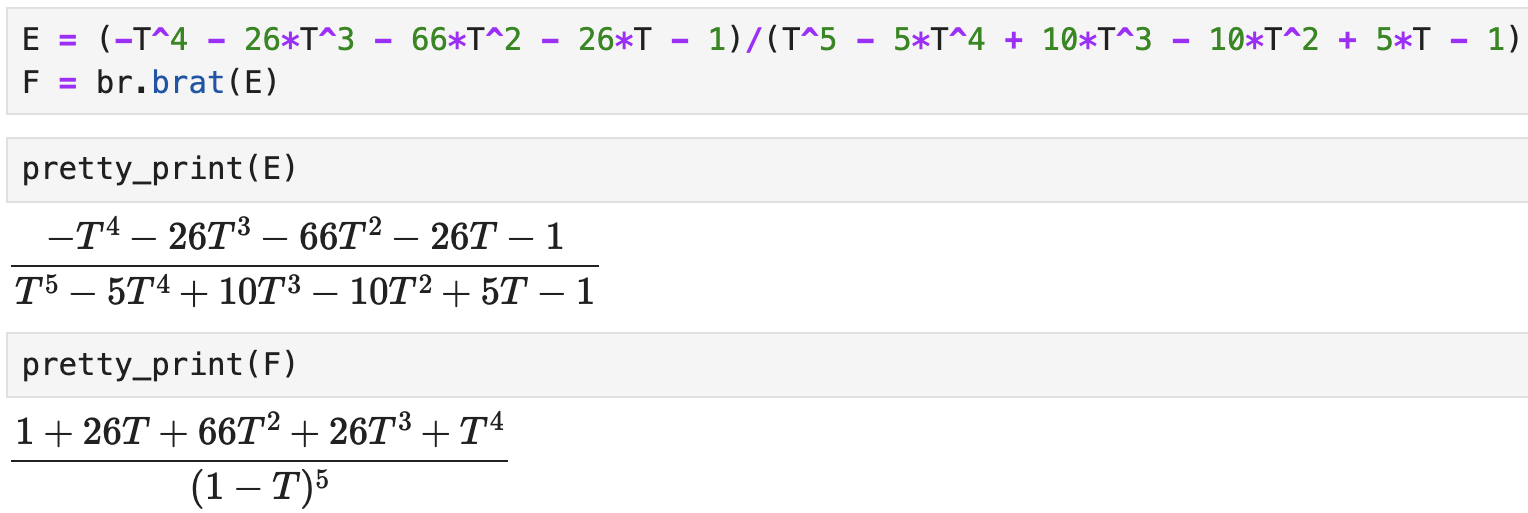
When applying the SageMath function pretty_print (or when it is on) in a Jupyter notebook, the brat will be displayed with $\LaTeX$.

There are many ways to set up a Jupyter notebook. One way is to run the following.

$ sage -n jupyter

In our Jupyter notebook, we observe the following.

Keys	Action
`?`	Open this help
`n`	Next page
`p`	Previous page
`s`	Search