Average Ehrhart coefficients & symplectic Hecke eigenbases

Joshua Maglione

How to Navigate:

Spacebar: Forward

Shift + Spacebar: Backward

Escape: Jump around

Arrow keys: Move around

Creative Commons Attribution 4.0

International License

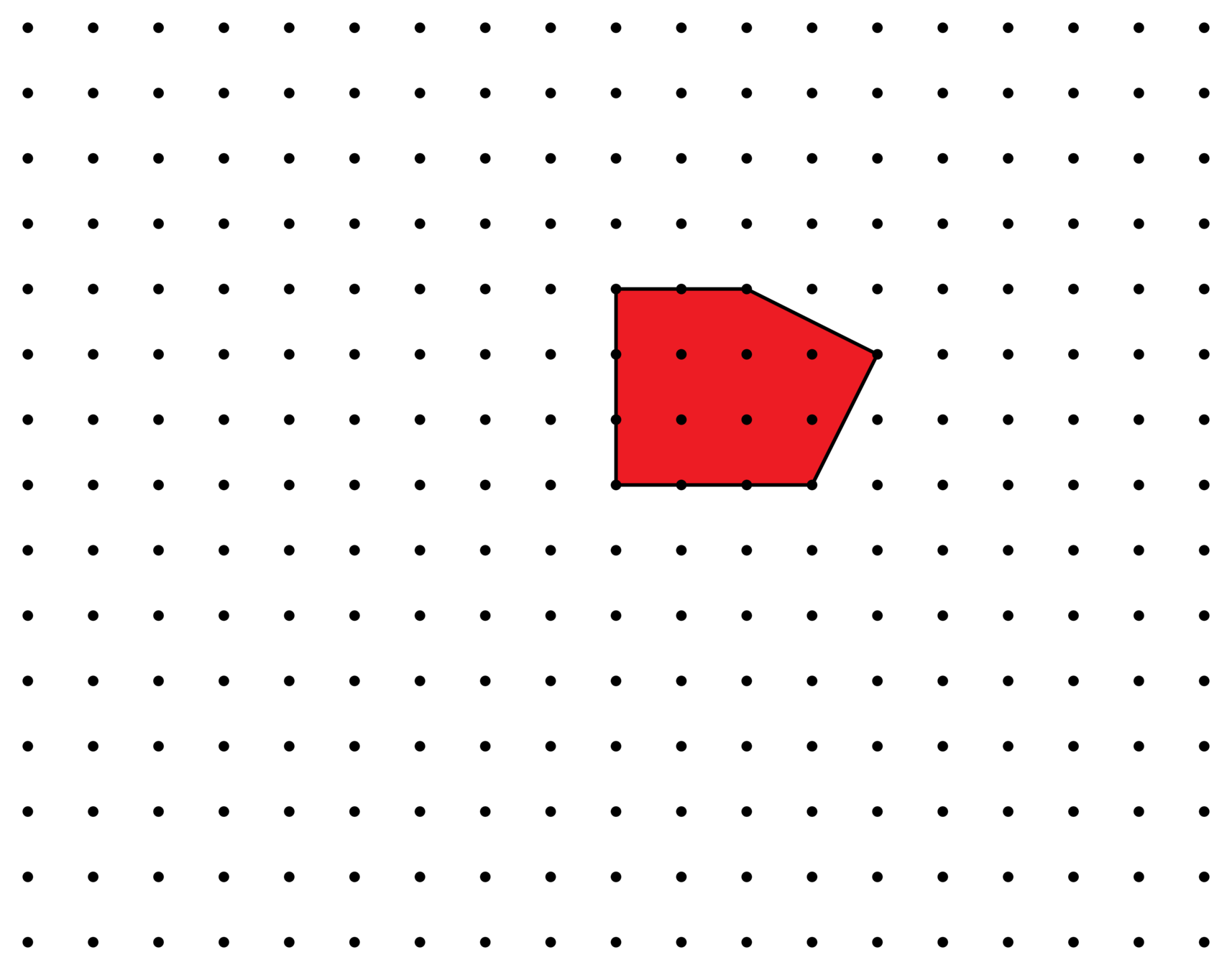
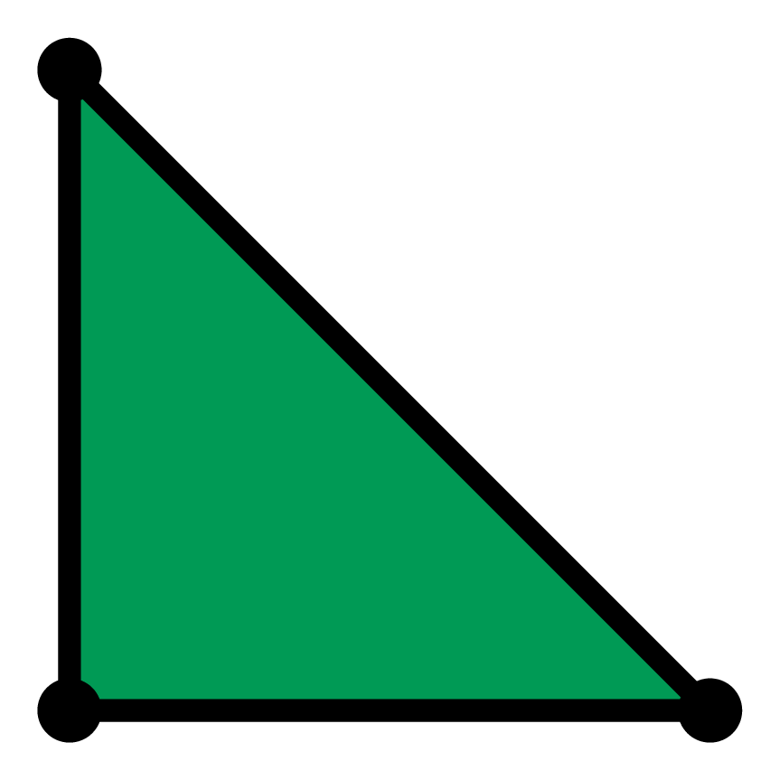
Polytopes

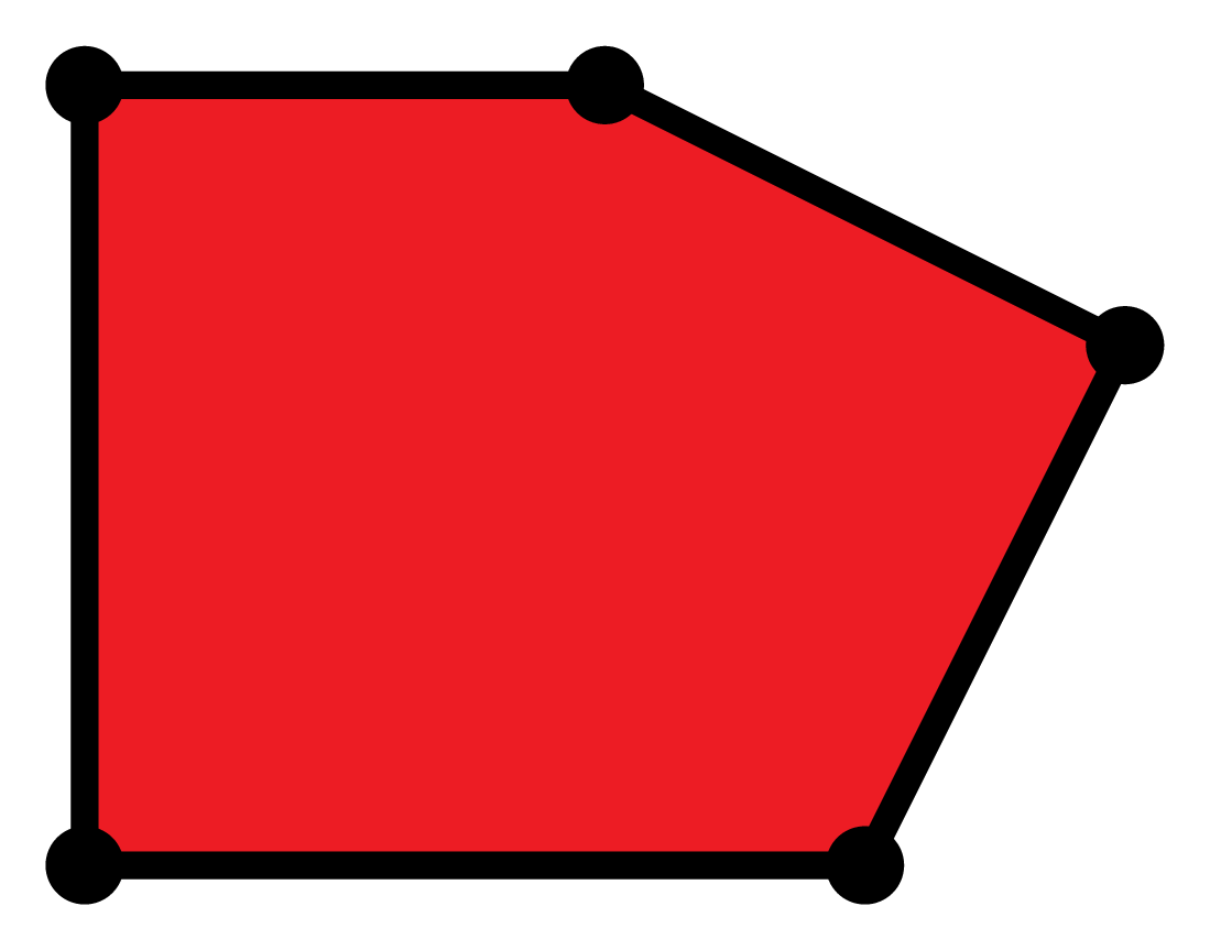
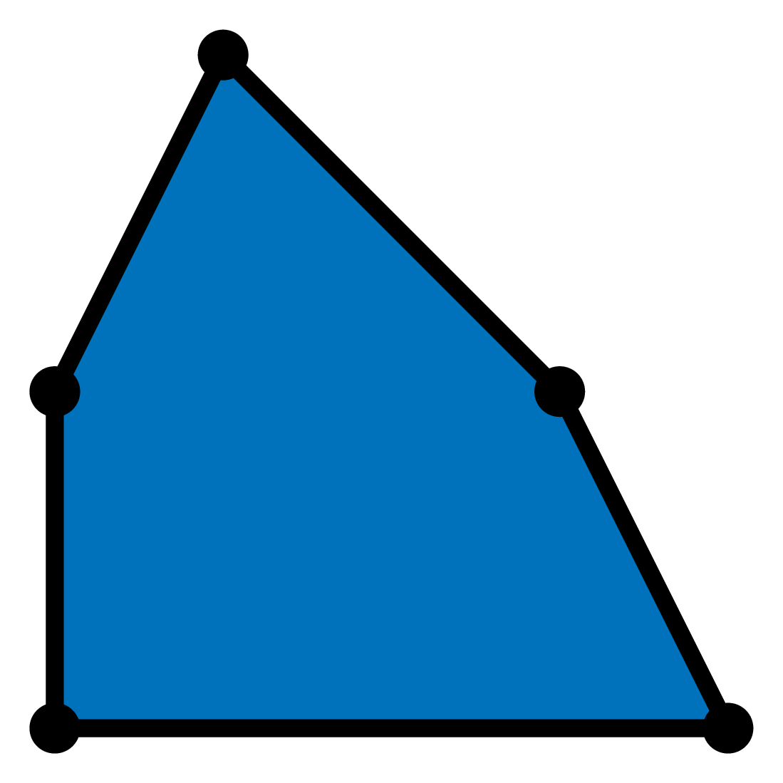
A polytope is the convex hull of finitely many points in $\mathbf{R}^n$.

A lattice polytope is the convex hull of finitely many points in $\mathbf{Z}^n\subset \mathbf{R}^n$.

For us: "polytope" means "lattice polytope"

Discrete Volumes

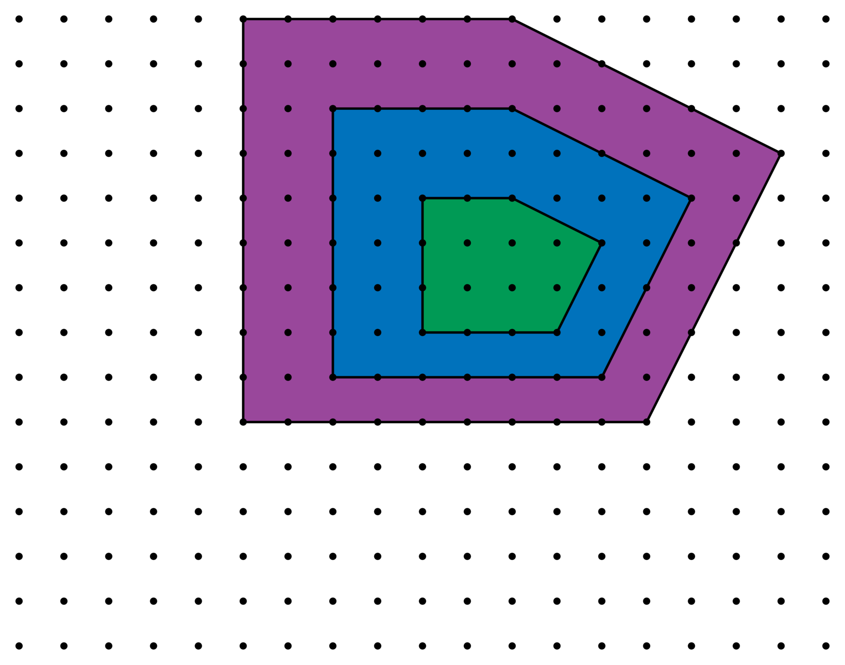
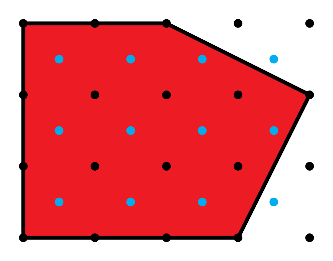
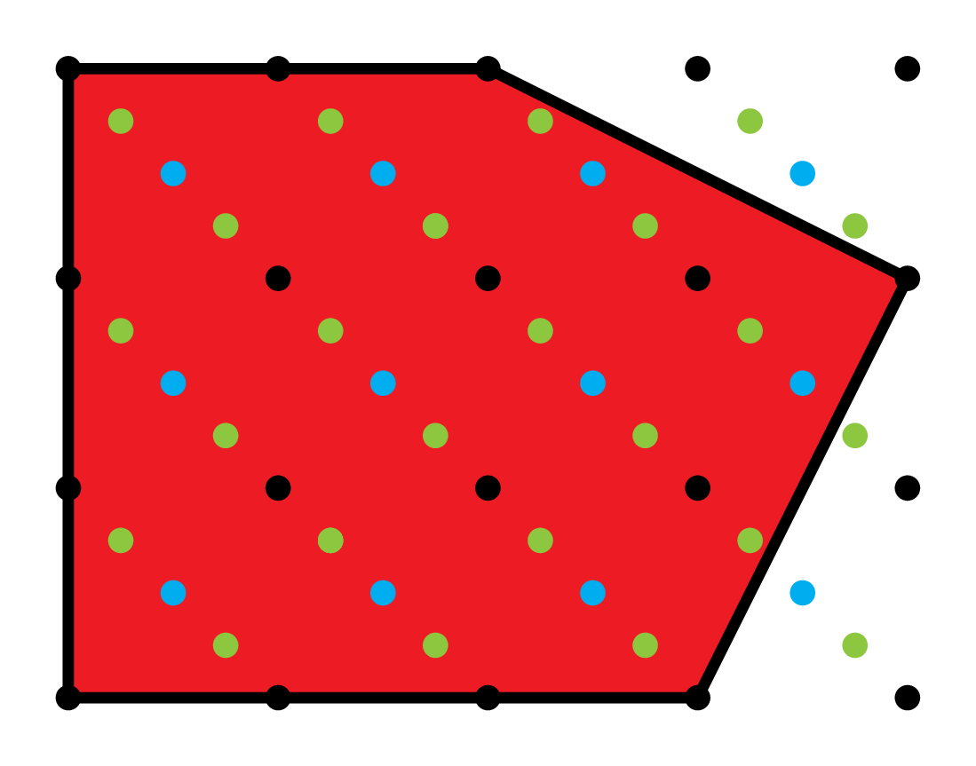
For a polytope $P$ and $k\in \mathbf{Z}_{\geqslant 0}$ the $k$th dilate is $kP = \{k\cdot p ~|~ p \in P\}$

The discrete volume of a polytope $P$ is $\# (P\cap \mathbf{Z}^n)$.

\lim_{k\to \infty} \dfrac{\#(kP\cap \mathbf{Z}^n)}{k^n} = \mathrm{vol}(P)

Theorem (Ehrhart (1962)). The function

is given by a polynomial (in $k$).

E_P : \mathbf{Z}_{\geqslant 0} \to \mathbf{Z}, \qquad k\mapsto \#(kP\cap\mathbf{Z}^n)

Corollary. The degree is $\leqslant n$. The coefficient of $t^n$ is $\mathrm{vol}(P)$.

Ehrhart

polynomial

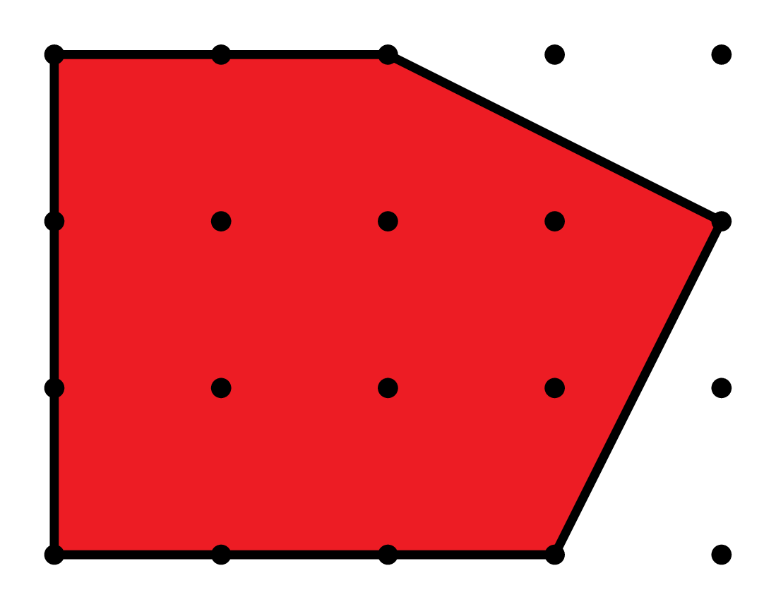
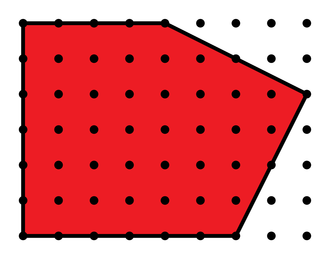
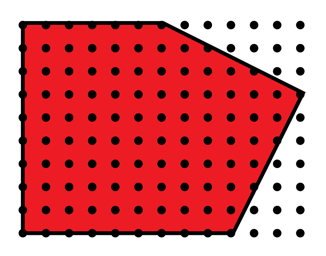
Ehrhart polynomials

$E(t) = 10t^2 + 5t + 1$

$E_P^{\Lambda}(t)$ : Ehrhart polynomial

$t \mapsto \#(tP\cap \Lambda)$

lattice: $\Lambda = \mathbf{Z}^2$

$E(1)=16$

$E(3)=106$

$E(2)=51$

Other coefficients with meaning?

Let $E_P^{\Lambda}(t) = c_0 + c_1t + \cdots + c_nt^n$. For $\ell\in \{0,\dots, n\}=[n]_0$, define

\mathscr{E}_{n, \ell}^{\Lambda}(P) = c_{\ell}.

Thus, $\mathscr{E}_{n,\ell}^{\Lambda}$ is the function on polytopes in $\mathbf{R}^n$ extracting the $\ell$th coefficient of its Ehrhart polynomial.

\begin{aligned} \mathscr{E}_{n,n} &= \mathrm{vol} \\ \mathscr{E}_{n,n-1} &= \frac{1}{2}\mathrm{vol}_{\partial} \\ &~~\vdots \\ \mathscr{E}_{n,0} &= 1 \end{aligned}

\Lambda = \mathbf{Z}^n

$\mathbf{Z}^n\subseteq \Lambda\subset \mathbf{Q}^n$

\begin{aligned} \mathscr{E}_{n,n}^{\Lambda} &= \mathrm{vol}_{\Lambda} \\ \mathscr{E}_{n,n-1}^{\Lambda} &= \frac{1}{2}\mathrm{vol}_{\Lambda,\partial} \\ &~~\vdots \\ \mathscr{E}_{n,0}^{\Lambda} &= 1 \end{aligned}

complicated

Example: $(a,b,c)$-simplex

\mathscr{E}_{3,0}(P) = 1 \qquad \mathscr{E}_{3,2}(P) = \frac{ab+bc+ca+1}{4} \qquad \mathscr{E}_{3,3}(P) = \frac{abc}{6}

(0,0,0)

(0,0,c)

(0,b,0)

(a,0,0)

P =

$(a,b,c)$ co-prime

Here, $S$ is a Dedekind sum. With

\mathscr{E}_{3,1}(P) = \frac{1}{12}\left(\frac{ab}{c} + \frac{bc}{a} + \frac{ca}{b} + \frac{1}{abc} + 3(a+b+c) + 9\right) - S

s(p, q) = \sum_{i=1}^q \left(\left(\frac{i}{q}\right)\right) \left(\left(\frac{pi}{q}\right)\right)

((x)) = \begin{cases} 0 & x\in \mathbf{Z}, \\ x - \lfloor x\rfloor -1/2 & x\not\in \mathbf{Z}, \end{cases}

S = s(ab, c) + s(bc, a) + s(ca, b)

Mordell (1951), Pommersheim (1993), Kantor & Khovanskii (1993)

Brion & Vergne (1997) proved that $\mathscr{E}_{n,\ell}$ are given by certain differential Todd operators acting on $\mathrm{vol}$ for simple polytopes.

\mathrm{Todd}(z) = \dfrac{z}{1 - \mathrm{exp}(-z)} = 1 + \frac{1}{2}z + \sum_{k=1}^{\infty}(-1)^{k-1}\dfrac{B_{2k}}{(2k)!}z^{2k}

Unimodular invariant valuations

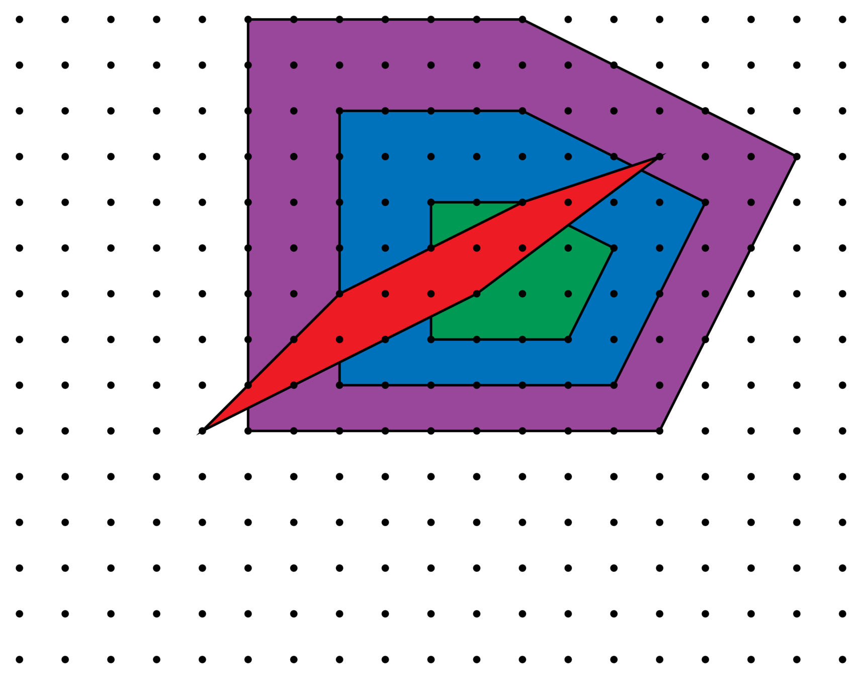
An $\mathbf{R}$-valued function $\varphi$ on polytopes is a valuation if

\varphi(P) + \varphi(Q) = \varphi(P\cup Q) + \varphi(P\cap Q)

whenever $P, Q, P\cap Q, P\cup Q$ are polytopes and $\varphi(\varnothing)=0$.

A valuation $\varphi$ is unimodular invariant if for all $\alpha\in \mathrm{Aut}(\Lambda)\!\leqslant\! \mathrm{Aff}_{n}(\mathbf{R})$

\varphi = \varphi\alpha.

Valuations capture

"geometric" measurements

Examples:

Volume
Surface area
Mean width
Euler characteristic

is a basis for the space of unimodular invariant valuations.

\left\{\mathscr{E}_{n,0},\; \mathscr{E}_{n,1},\; \dots,\; \mathscr{E}_{n,n}\right\}

Theorem (Betke & Kneser (1985)). The set

The Ehrhart coefficients encode all geometric measurements.

Betke & Kneser is a discrete analogue of Hadwiger's Theorem (1957).

The analogy, unfortunately, does not carry over to the properties of the valuations $\mathscr{E}_{n,\ell}$.

The $n+1$ intrinsic volumes are a basis for the space of certain valuations on compact convex bodies in $\mathbf{R}^n$.

\sum_{m=0}^{\infty} E_P(m) t^m = \dfrac{h^*_0(P) + h^*_1(P)t + \cdots + h^*_n(P)t^n}{(1 - t)^{n+1}}

We can form the Ehrhart series:

Ehrhart series & $h^*$-polynomial

The $h_i^*$ are unimodular invariant but not valuations.

Stanley (1980) proved non-negativity:

\begin{aligned} h_0^*(P) &= 1, & h_k^*(P) &\in \mathbf{Z}_{\geqslant 0} \end{aligned}

and, in (1993), monotonicity:

P\subseteq Q \implies \forall i,\ h_i^*(P)\leqslant h_i^*(Q)

Is there anything special about Ehrhart coefficients?

\sum_{i=0}^n{\color{blue}\mathscr{E}_{n,i}(P)}t^i = \sum_{i=0}^n {\color{blue}h_i^*(P)} \binom{t + n - i}{n} = \sum_{i=0}^n {\color{blue}f_i^*(P)} \binom{t - 1}{i}

Breuer (2012) defined the $f^*$-polynomial writing Ehrhart polynomial in a different polynomial basis:

Jochemko & Sanyal (2018) proved that the $f^*_i$ form the essentially unique basis for $\mathrm{UIV}_n$ which are non-negative and monotone.

unimodular invariant

valuations

Unique* Hecke eigenfunctions

Theorem (Alfes, M, & Voll (2025)). The valuations

\{\mathscr{E}_{2n,0}, \mathscr{E}_{2n, 1}, \dots, \mathscr{E}_{2n, 2n}\}

form a symplectic Hecke eigenbasis for the space of $\mathrm{UIV}_{2n}$.

Theorem (Gunnells & Rodriguez Villegas (2007)). The valuations

\{\mathscr{E}_{n,0}, \mathscr{E}_{n, 1}, \dots, \mathscr{E}_{n, n}\}

form a Hecke eigenbasis for the space of $\mathrm{UIV}_n$.

Up to independent scaling, this is the unique basis of such valuations.

Lattice perspective

$\mathbf{Z}^n$

$\frac{1}{2}\mathbf{Z}^n$

$\frac{1}{3}\mathbf{Z}^n$

\#(kP \cap \mathbf{Z}^n) = \#(P \cap \tfrac{1}{k}\mathbf{Z}^n)

Consider how $\mathscr{E}_{n,\ell}^{\Lambda}$ changes as we refine $\mathbf{Z}^n\subseteq \Lambda\subset \mathbf{Q}^n$.

Represent a lattice $\Lambda$ by a matrix, whose rows generate $\Lambda$.

\mathbf{Z}^2 \leftrightsquigarrow \begin{pmatrix} 1 & 0 \\ 0 & 1 \end{pmatrix}

Lattices $\Lambda\supseteq\mathbf{Z}^2$

\Lambda = 2^{-1}\left(\begin{smallmatrix} \phantom{0} & \phantom{0} \\ \phantom{0} & \phantom{0} \end{smallmatrix}\right)

\Lambda = 4^{-1}\left(\begin{smallmatrix} \phantom{0} & \phantom{0} \\ \phantom{0} & \phantom{0} \end{smallmatrix}\right)

\Lambda \mapsto \mathcal{E}_{2, 1}^{\Lambda}(\phantom{poly})

\begin{aligned} \mathrm{conv}&\{(0,0), (0,3), (2,3),\\ &\;(3,0), (4,2)\} \end{aligned}

\begin{aligned} \mathrm{conv}&\{(0,0), (0,2), (1,4),\\ &\;(3,2), (4,0)\} \end{aligned}

\begin{aligned} \mathrm{conv}&\{(0,0), (0,1), (1,0)\} \end{aligned}

Normalized sums of coefficients

Fix a polytope $P$, with $\mathscr{E}_{n,\ell}(P)\neq 0$. Define

where $\Lambda\supseteq\mathbf{Z}^n$ runs over all lattices in $\mathbf{Q}^n$ with $\#(\Lambda/\mathbf{Z}^n)=m$.

Just as a lattice generated from a matrix from $\mathrm{GL}_n(\mathbf{Q})\cap\mathrm{Mat}_n(\mathbf{Z})$,

a symplectic lattice is generated from one in $\mathrm{GSp}_{2n}(\mathbf{Q})\cap\mathrm{Mat}_{2n}(\mathbf{Z})$.

\mathcal{C}_{P,\ell}^{\mathsf{A}} : \mathbf{N} \longrightarrow \mathbf{Q}

m \longmapsto \dfrac{1}{\mathscr{E}_{n,\ell}(P)} \sum_{\Lambda} \mathscr{E}_{n,\ell}^{\Lambda}(P),

Define $\mathcal{C}_{P,\ell}^{\mathsf{C}} : \mathbf{N}\to \mathbf{Q}$ similarly but restricted to symplectic lattices.

We computed $\mathcal{C}_{P,1}^{\mathsf{A}}(2)$ and $\mathcal{C}_{P,1}^{\mathsf{A}}(4)$.

An arithmetic function

Write $\mathsf{X}$ for either $\mathsf{A}$ or $\mathsf{C}$.

Theorem (Alfes, M, & Voll (2025)).

(Independence) For polytopes $P$ and $Q$, with $\dim P=\dim Q$,

(Multiplicativity) For $a,b\in \mathbf{N}$ with $\mathrm{gcd}(a,b)=1$,

\mathcal{C}_{P,\ell}^{\mathsf{X}}(ab) = \mathcal{C}_{P,\ell}^{\mathsf{X}}(a)\mathcal{C}_{P,\ell}^{\mathsf{X}}(b).

\mathcal{C}_{P,\ell}^{\mathsf{X}}=\mathcal{C}_{Q,\ell}^{\mathsf{X}}.

Growth rate of coefficients

For functions $f,g : \mathbb{R}\to \mathbb{R}$, we write

f(N) \sim g(N) \quad \iff \quad \lim_{N\to \infty} \dfrac{f(N)}{g(N)} = 1.

Proposition (Alfes, M, & Voll (2025)).

Let $\ell\in \{0,1,\dots, n\}$. Assuming $\mathscr{E}_{n,\ell}(P)\neq 0$,

\sum_{m=1}^{N} \mathcal{C}_{P,\ell}^{\mathsf{A}}(m) \,\sim\, \begin{cases} \frac{\zeta(n-\ell)}{n} \zeta(2)\zeta(3) \cdots \zeta(n-1) N^n & \text{if }\ell\leqslant n-2, \\[0.5em] \frac{1}{n}\zeta(2)\zeta(3) \cdots \zeta(n-2) N^n \log N & \text{if }\ell=n-1, \\[0.5em] \frac{1}{n+1} \zeta(2)\zeta(3) \cdots \zeta(n) N^{n+1} & \text{if }\ell=n. \end{cases}

Here, $\zeta$ is the Riemann zeta function.

Averaging over all lattices

Corollary.

Let $P$ be an $n$-dimensional polytope in $\mathbf{Z}^n$ and $\ell\in \{0,1,\dots, n-2\}$. The average $\ell$th Ehrhart coefficient of $P$, running over all $\Lambda\supseteq\mathbf{Z}^n$ in $\mathbf{Q}^n$ with finite co-index, approaches

\dfrac{\zeta(n-\ell)}{\zeta(n)} \mathscr{E}_{n,\ell}(P).

Example. For $n=3$, the average linear coefficient approaches

\dfrac{\pi^2}{6\zeta(3)}\mathscr{E}_{3,1}(P) \approx 1.37\cdot\mathscr{E}_{3,1}(P)

Example. For $n=4$, the average quadratic coefficient approaches

\dfrac{15}{\pi^2}\mathscr{E}_{4,2}(P) \approx 1.52\cdot \mathscr{E}_{4,2}(P)

Growth rate (symplectic edition)

Theorem (Alfes, M, & Voll (2025)).

For each $\ell\in \{0,1,\dots, 2n\}$ there exists $c_{n,\ell}\in\mathbb{R}$ such that

\sum_{m=1}^{N}\mathcal{C}_{P,\ell}^{\mathsf{C}}(m) \,\sim\, c_{n,\ell}\sqrt{N^{n+1}}\sqrt[n]{N^{\max(0,\ell-n)+1}}(\log N)^{\delta_{n,\ell}}

For $i,j\in\mathbb{N}_0$, write $\delta_{i,j}$ for the Kronecker delta symbol.

For $n=2$ (i.e. in $4$ dimensions) we completely know $c_{2,\ell}$:

\begin{aligned} c_{2,0} &= \frac{7\zeta(3)}{8}, & c_{2,1} &= \frac{\zeta(2)^2\zeta(3)}{12\zeta(5)}, & c_{2,2} &= \frac{5}{8}, & c_{2,3} &= \frac{2\zeta(2)^2\zeta(3)}{5\zeta(5)}, & c_{2,4} &= \frac{7\zeta(3)}{12}. \end{aligned}

Averaging over symplectic lattices

When $n=2$ and $\ell=1$, the average linear coefficient is

Corollary.

Let $P$ be $2n$-dimensional in $\mathbf{Z}^{2n}$. The average $\ell$th Ehrhart coefficient, running over all symplectic lattices, converges only when $\ell\in\{0,1,\dots, n-1\}$. Its limit is

\dfrac{c_{n,\ell}}{c_{n,0}} \mathscr{E}_{2n,\ell}(P).

\dfrac{\pi^4}{63\zeta(5)}\mathscr{E}_{4,1}(P) \approx 1.49 \cdot \mathscr{E}_{4,1}(P).

Modular form analogue

Previous theorems stem from the understanding extracted from the Hecke operators.

CC BY-SA 4.0 Kilom691

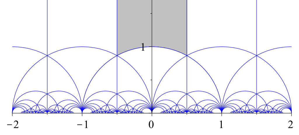
Points in $\mathrm{SL}_2(\mathbf{Z})\setminus \mathbf{H}$

$\mathrm{GL}_n(\mathbf{Z})\setminus\{\text{Polytopes}\}$

Modular form weight $k$

$\mathscr{E}_{n,k}$

\leftrightsquigarrow

\begin{aligned} G^+ &= \mathrm{GSp}_{2n}(\mathbf{Q}_p)\cap \mathrm{Mat}_{2n}(\mathbf{Z}_p), & \Gamma &= \mathrm{GSp}_{2n}(\mathbf{Z}_p) \end{aligned}

The (symplectic) Hecke ring $\mathcal{H}$ is the set of functions $G^+ \to \mathbf{Z}$ that:

are continuous (thus, locally constant),
have compact support,
are constant on $\Gamma$-double cosets.

$\mathbf{Z}$-basis for $\mathcal{H}$ : characteristic functions on $\Gamma$-double cosets.

\mathcal{H} = \mathbf{Z}[T_0, T_1, \dots, T_n].

\begin{aligned} D_0 &= \begin{pmatrix} I_n & \\ & pI_n \end{pmatrix}, & D_k &= \begin{pmatrix} I_{n-k} & & & \\ & pI_k & & \\ & & p^2I_{n-k} & \\ & & & pI_k \end{pmatrix}. \end{aligned}

We define matrices $D_0,\dots, D_n\in G^+$: for $k\in \{1,\dots, n\}$,

Let $T_k\in\mathcal{H}$ be the characteristic function on $\Gamma D_k\Gamma$. Thus,

(symplectic)

elemtary

divisors

For $f\in\mathrm{UIV}_{2n}$, define $Tf\in\mathrm{UIV}_{2n}$ via

where

$\Gamma\setminus \Gamma g \Gamma$ : set of lattices with prescribed elementary divisors,

Extend linearly to define an action of $\mathcal{H}$ on $\mathrm{UIV}_{2n}$.

Let $T\in\mathcal{H}$ be the characteristic function for $\Gamma g\Gamma$, so associated with some elementary divisors.

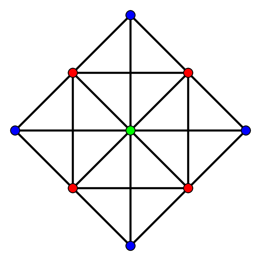
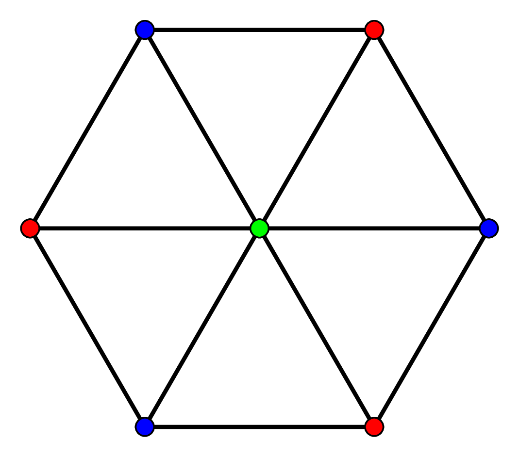
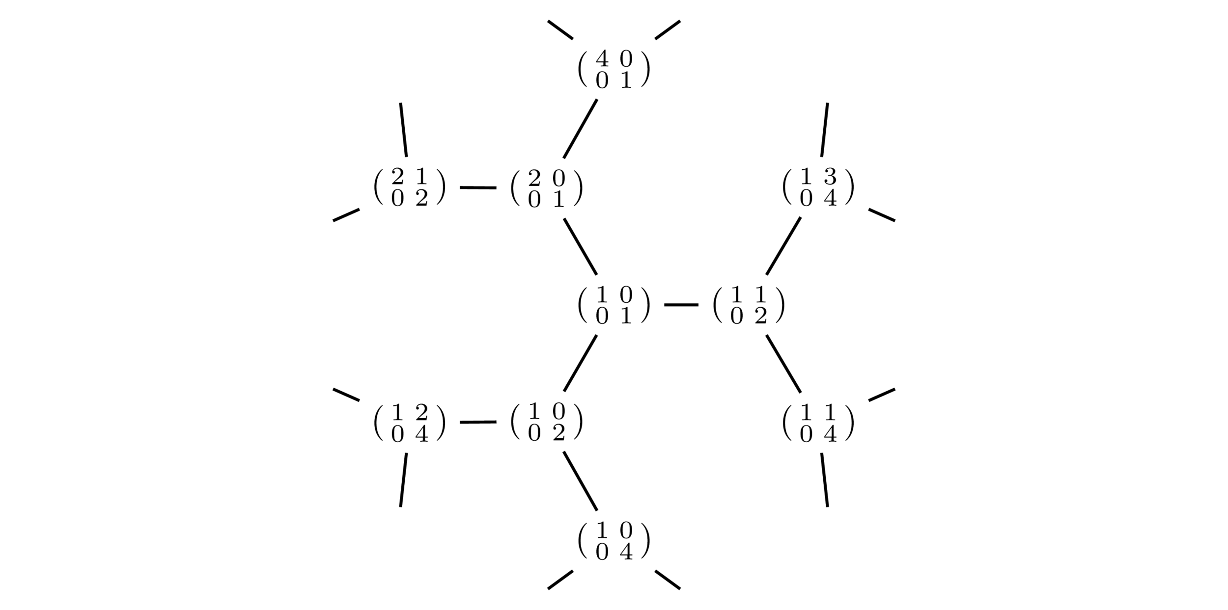
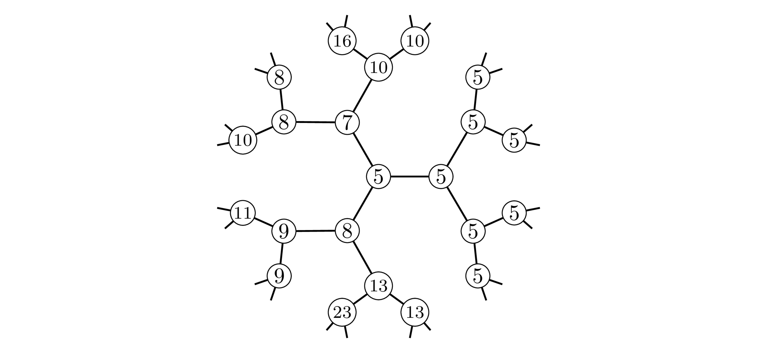
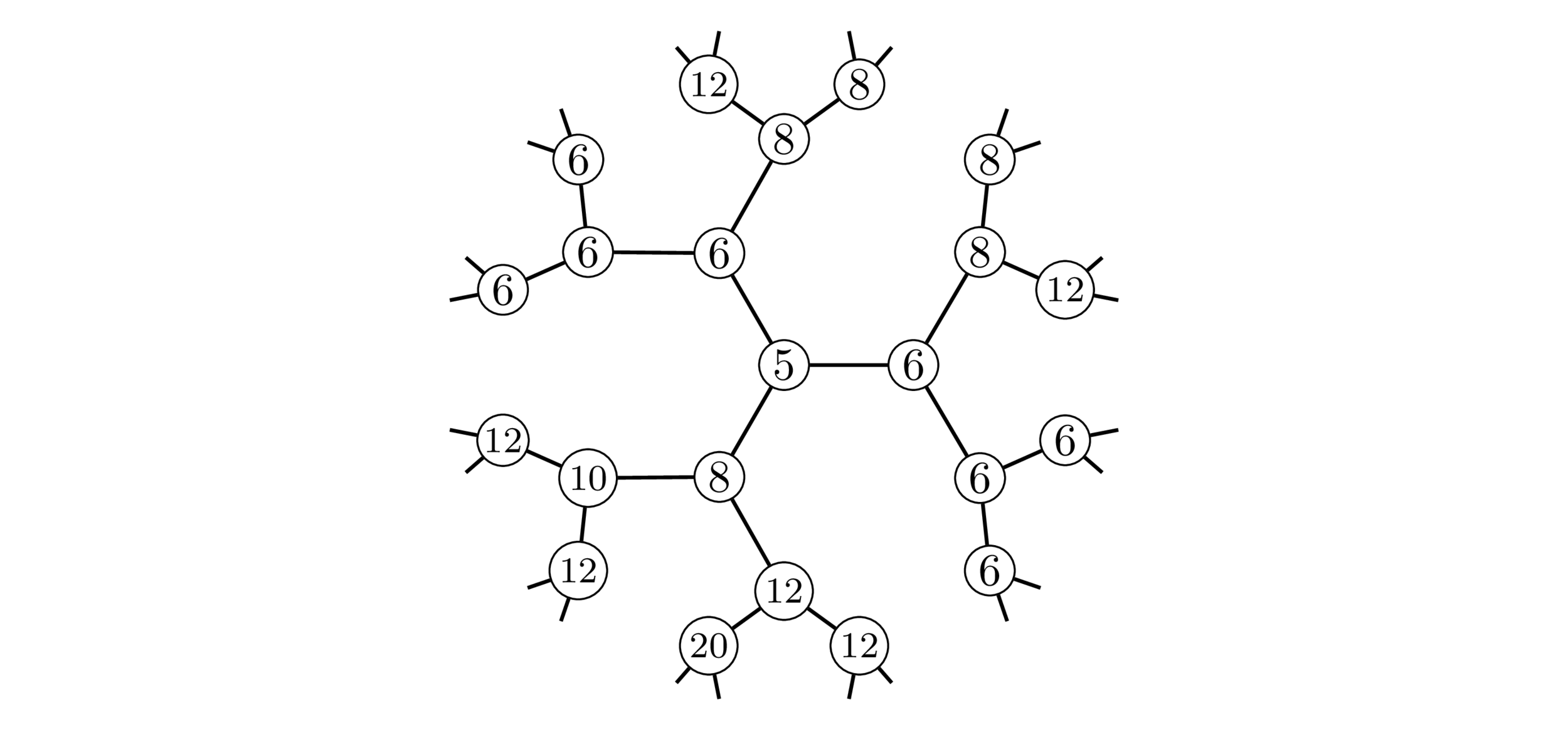
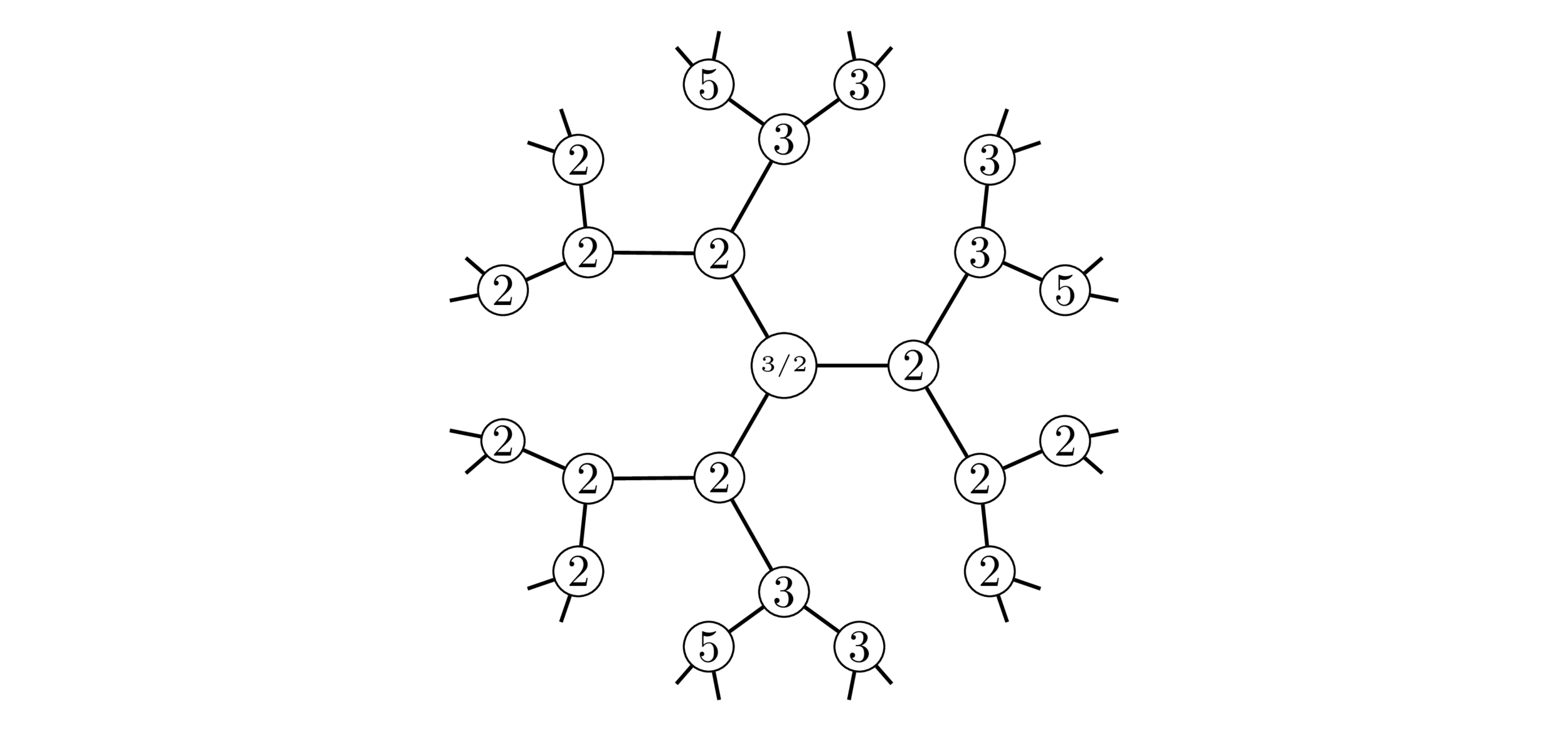
What does this action look like on our generators $T_k$?

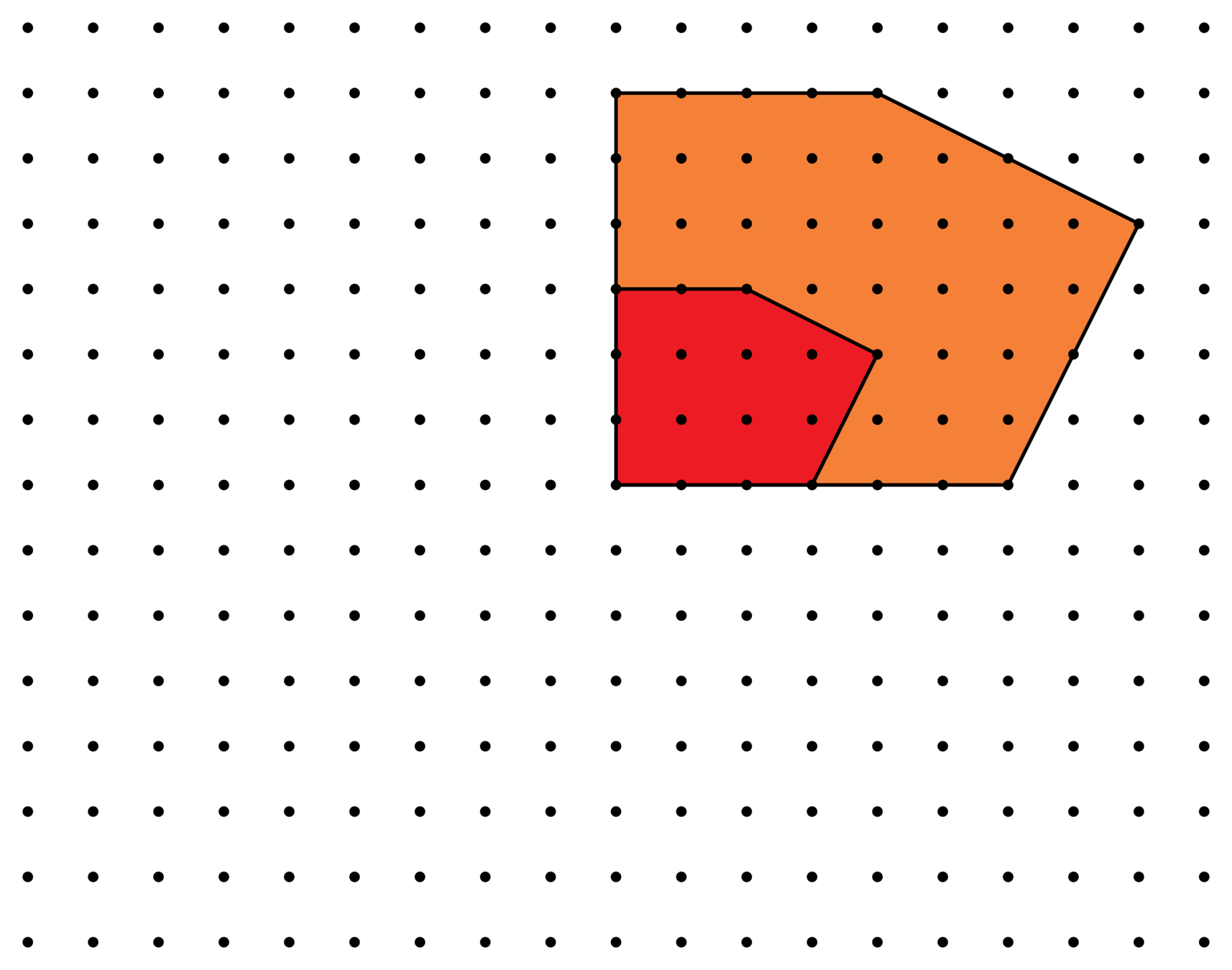
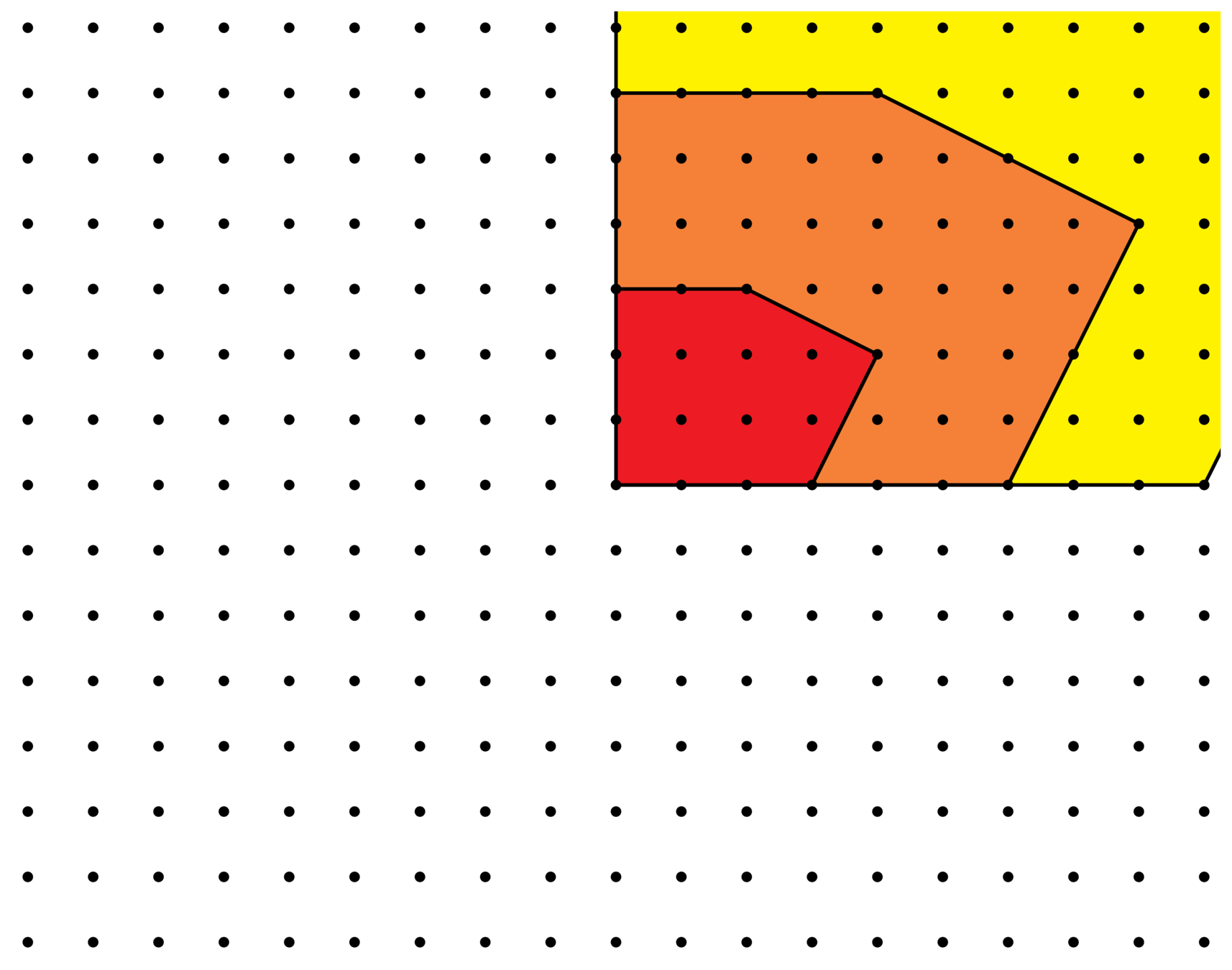
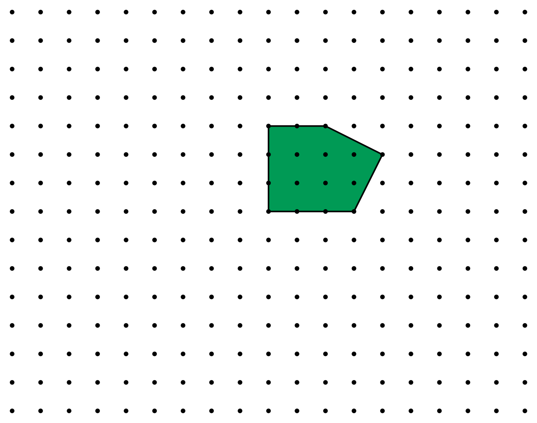
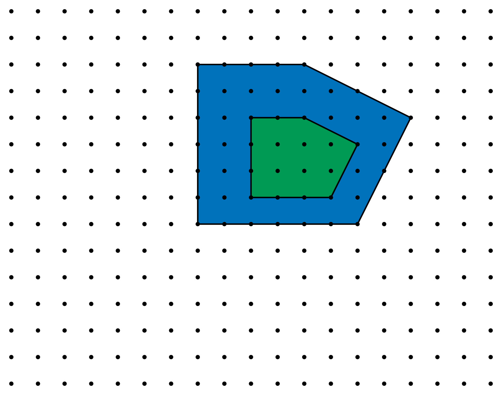
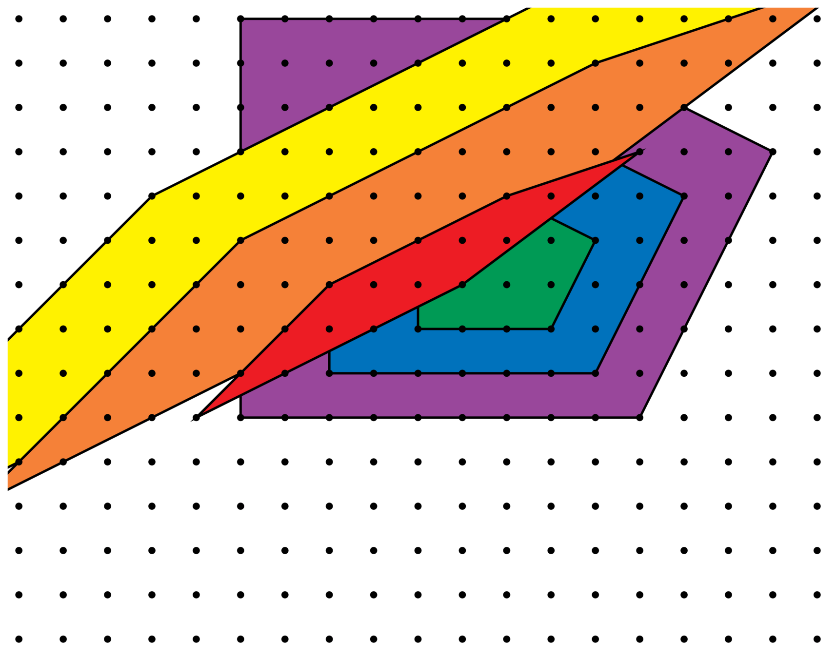
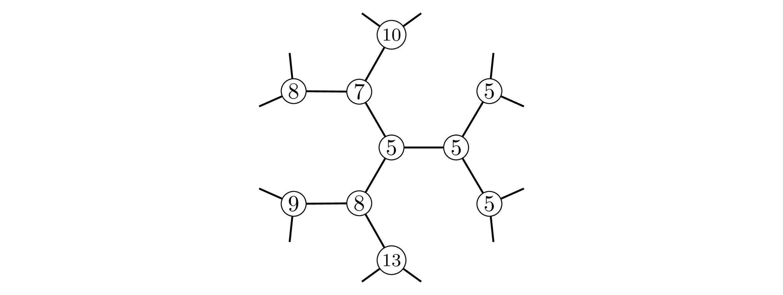
Tf(P) = \sum_{\Gamma h \,\in\, \Gamma \setminus \Gamma g\Gamma} f(h\cdot P)

$h\cdot P$ : given by some integer matrix in $\Gamma h$ acting on vertices.

Each matrix corresponds to a $\Gamma$-left coset.

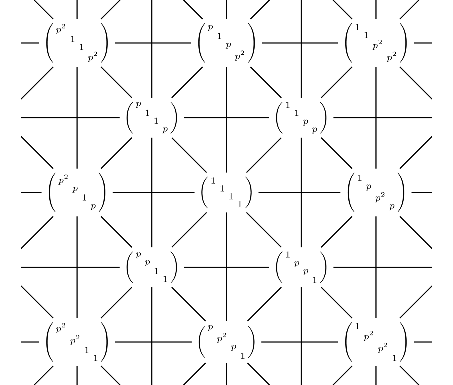
Colors correspond to $\Gamma$-double cosets.

\Gamma\begin{pmatrix} 1 \\ &1 \\ &&p \\ &&&p \end{pmatrix}\Gamma

T_0

\Gamma\begin{pmatrix} 1 \\ &p \\ &&p^2 \\ &&&p \end{pmatrix}\Gamma

T_1

\Gamma\begin{pmatrix} p \\ &p \\ &&p \\ &&&p \end{pmatrix}\Gamma

T_2

Knowing that the $\mathscr{E}_{2n,\ell}$ form a symplectic Hecke eigenbasis means we can take advantage of the theory of spherical functions.

Leads to a nice interpretation of the associated zeta function:

\mathcal{Z}_{n,\ell,p}^{\mathsf{X}}(s) = \sum_{\Gamma g \,\in\, \Gamma\setminus \Gamma G^+\Gamma} \dfrac{\mathscr{E}_{2n,\ell}(g\cdot P)}{\mathscr{E}_{2n,\ell}(P)} \left|\Lambda_{g} : \Lambda_0\right|^{-s}.

Ehrhart–Hecke zeta functions

Lattice

from $\Gamma g$

To understand growth of $\mathcal{C}_{P,\ell}^{\mathsf{X}}$, need to understand $\mathcal{Z}_{n,\ell,p}^{\mathsf{X}}$ for all $p$:

\mathcal{Z}_{n,\ell}^{\mathsf{X}}(s) := \sum_{m=1}^{\infty} \mathcal{C}_{P,\ell}^{\mathsf{X}}(m)\, m^{-s} = \prod_{p\text{ prime}} \mathcal{Z}_{n,\ell,p}^{\mathsf{X}}(s)

Main method of proof: lattice enumeration from M & Voll (2024).

\mathcal{Z}_{n,\ell}^{\mathsf{A}}(s) = \zeta(s - \ell) \cdot \zeta(s - 1) \zeta(s-2)\cdots \zeta(s - n + 1)

Type A case is simpler. We know the global zeta function:

\mathcal{Z}_{n,\ell,p}^{\mathsf{C}}(s) = \sum_{I,J\subseteq [n]} \Psi_{n,I,J}(p^{-1}) \prod_{i\in I} \dfrac{p^{\binom{i+1}{2} + i(n-i)}t^n}{1-p^{\binom{i+1}{2} + i(n-i)}t^n} \prod_{j\in J} \dfrac{p^{\binom{j+1}{2} + j(n-j) - n + \ell}t^n}{1-p^{\binom{j+1}{2} + j(n-j) - n + \ell}t^n}

Theorem (Alfes, M, & Voll (2025)).

Setting $t = p^{-s}$,

\Psi_{n,I,J}(Y) = \text{$Y$-multinomial coefficient} \times \prod (1 - Y^k)^{e_k}

Type C case is more subtle. We know the local zeta function:

Summary

The $\mathscr{E}_{2n,\ell}$ form a symplectic Hecke eigenbasis of $\mathrm{UIV}_{2n}$.

Theory of spherical functions on $p$-adic groups provide tools to study growth of coefficients.

Thank you!

Unique* valuations with this property

is $\zeta(n-\ell)/\zeta(n)$ for $\ell\in\{0,\dots, n-2\}$ over all lattices,

The average $\ell$th coefficient of the Ehrhart polynomial...

converges for $\ell\in \{0,\dots, \frac{2n}{2} - 1\}$ over sympletic lattices.

Average Ehrhart coefficients & symplectic Hecke eigenbases

Polytopes

Discrete Volumes

Ehrhart polynomials

Other coefficients with meaning?

Example: \((a,b,c)\)-simplex

Unimodular invariant valuations

Ehrhart series & \(h^*\)-polynomial

Unique* Hecke eigenfunctions

Lattice perspective

Normalized sums of coefficients

An arithmetic function

Growth rate of coefficients

Averaging over all lattices

Growth rate (symplectic edition)

Averaging over symplectic lattices

Modular form analogue

Ehrhart–Hecke zeta functions

Summary

Thank you!