Igusa zeta functions and hyperplane arrangements
Joshua Maglione

How to Navigate:

Spacebar: Forward

Shift + Spacebar: Backward

Escape: Jump around

Arrow keys: Move around

The Igusa zeta function

Let \(f\in \mathbb{Z}[x_1, \dots, x_d]\). For every positive integer \(n\): 

R(n) = \#\left\{a \in \left(\mathbb{Z}/n\mathbb{Z}\right)^d ~\middle|~ f(a) \equiv 0\; (\text{mod }n) \right\}
  • Can we write a formula for \(R(n)\)?

If \(n = p_1^{e_1} \cdots p_{\ell}^{e_{\ell}}\) is the prime factorization of \(n\), then 

R(n) = R(p_1^{e_1}) \cdots R(p_{\ell}^{e_{\ell}})

So we focus on a prime \(p\).

  • How does \(R(p_i^{e_i})\) vary as \(i\) varies?
  • How does \(R(n)\) grow as \(n\) grows?
  • Only finitely many different formulae for the \(R(p^e)\) over all primes \(p\)?

We focus on polynomials equal to product of linear factors.

\begin{array}{r|cccc} e & 1 & 2 & 3 & 4 & 5 & 10\\ \hline R(p^e) & {\color{blue}9}p^2 & {\color{blue}22}p^4 & {\color{blue}7}p^7 & {\color{blue}3}p^{{\color{blue}10}} & {\color{blue}13}p^{12} & {\color{blue}9}p^{{\color{blue}26}} \end{array}

Leading terms!

\begin{array}{r|cccc} e & 1 & 2 & 3 & 4 & 5 & 10\\ \hline R(p^e) & {\color{blue}6}p^2 & {\color{blue}13}p^4 & {\color{blue}4}p^7 & {\color{blue}13}p^{{\color{blue}9}} & p^{12} & {\color{blue}13}p^{{\color{blue}24}} \end{array}

Theorem (Igusa 1974). 

  • The \(R(p^e)\) grow like a polynomial,
  • only finitely many different formulae for \(R(p^e)\), and
  • there is a finite linear recurrence relation among \(R(p^{e_i})\).

Example.
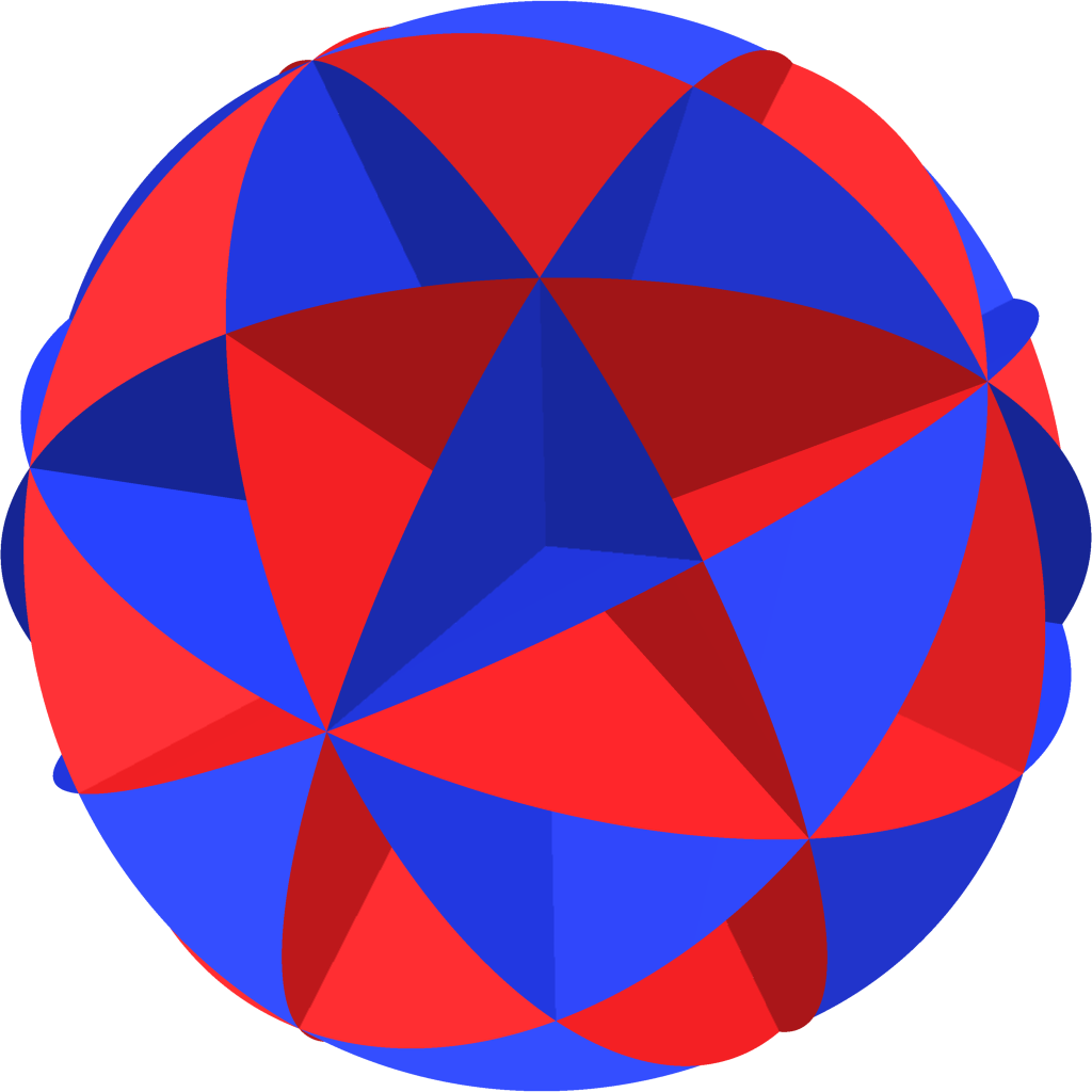
f = x_1x_2x_3(x_1^2 - x_2^2)(x_1^2 - x_3^2)(x_2^2 - x_3^2)
  • \(p >2\)
  • \(p =2\)

Overview

Understand features of Igusa zeta function with combinatorial & topological tools

flag Hilbert–Poincaré series

Igusa zeta function

combinatorial "coarsening"

Define flag Hilbert–Poincaré series and give substitution.

Hyperplane arrangements

Hyperplane arrangement \(\mathcal{A}\) finite set of hyperplanes in \(K^d\).

Intersection poset: ordered by reverse inclusion

\mathcal{L}(\mathcal{A}) = \left\{\bigcap_{H\in S} H ~\middle|~ S\subseteq \mathcal{A} \right\}.
  • Bottom element \(\hat{0}\) : the vector space \(K^d\).
  • Top element \(\hat{1}\) : the common intersection (if exists).

If \(\hat{1}\in\mathcal{L}(\mathcal{A})\), then \(\mathcal{A}\) is central.

\pi_{\mathcal{A}}(Y) = \displaystyle\sum_{x\in\mathcal{L}(\mathcal{A})} |\mu(\hat{0},x)|\cdot Y^{\mathrm{codim}(x)} = \mathrm{Poin}(\mathbb{C}^d \setminus \bigcup_{H\in\mathcal{A}}H;\; Y)

Poincaré polynomial:

Coefficients are Betti numbers.

Example.

\displaystyle\mathsf{A}_n = \prod_{1\leqslant i < j \leqslant n+1} (x_i - x_j).
\pi_{\mathsf{A}_3}(Y) = 1 + 6Y + 11Y^2 + 6Y^3

\(\mathrm{codim}\)

0

1

2

3

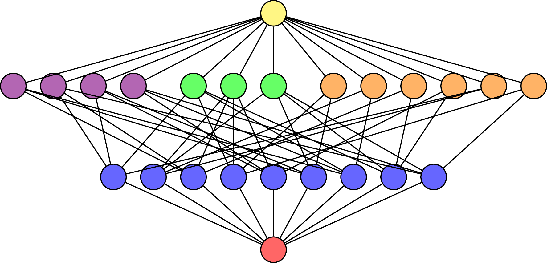
\(\mathcal{L}(\mathsf{A}_3)\)
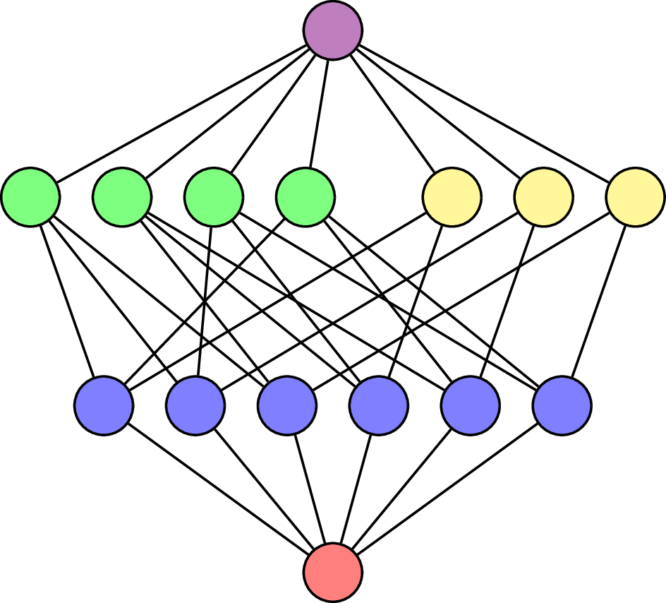
\(\hat{0}\)

\(\hat{1}\)
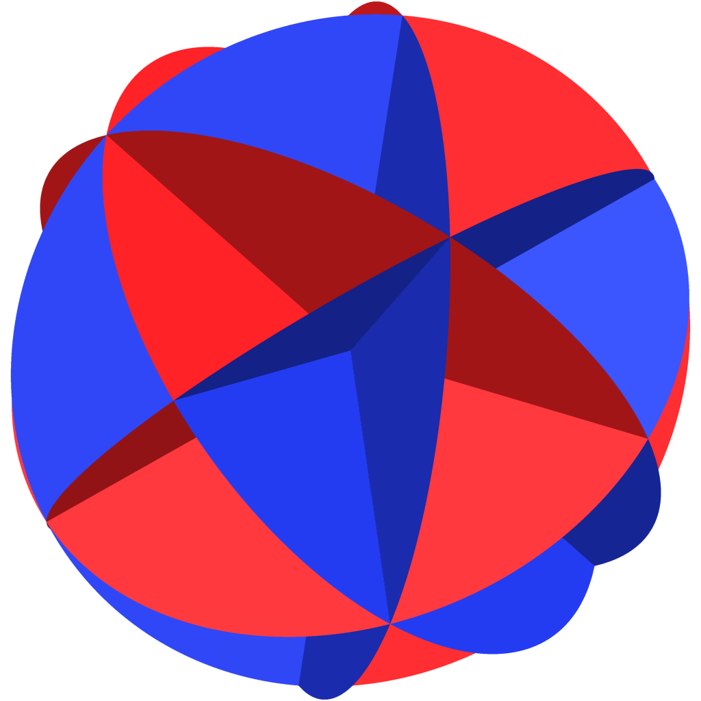
\(\mathsf{A}_3\)

\(K\!=\!\mathbb{C}\)

Write \(\Delta(\mathcal{L}(\mathcal{A})\setminus \{\hat{0}\})\) for flags of proper subspaces in \(\mathcal{L}(\mathcal{A})\).

For flag \(F = (F_1< \cdots <F_{\ell}) \in \Delta(\mathcal{L}(\mathcal{A})\setminus \{\hat{0}\})\), generalize:
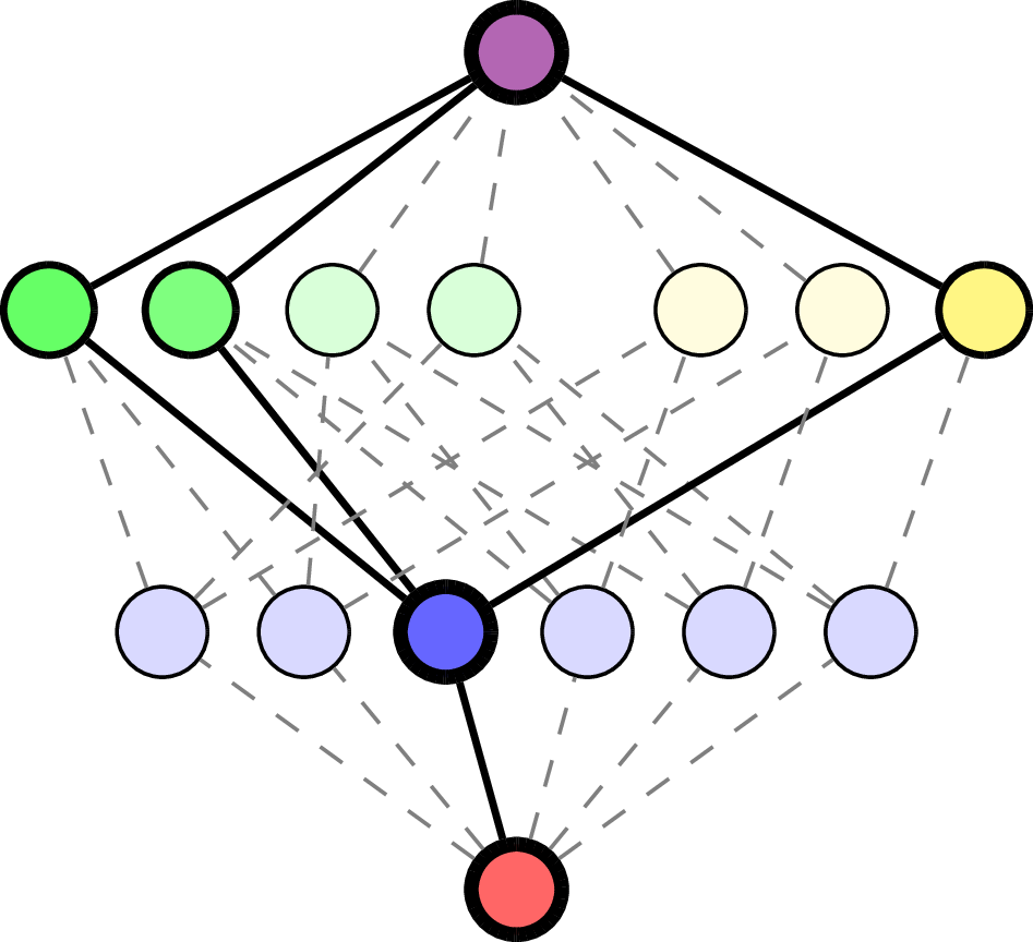
\pi_F(Y) = \pi_{[\hat{0},F_1]}(Y) \pi_{[F_1, F_2]}(Y) \cdots \pi_{[F_{\ell}, \hat{1}]}(Y)

Example.

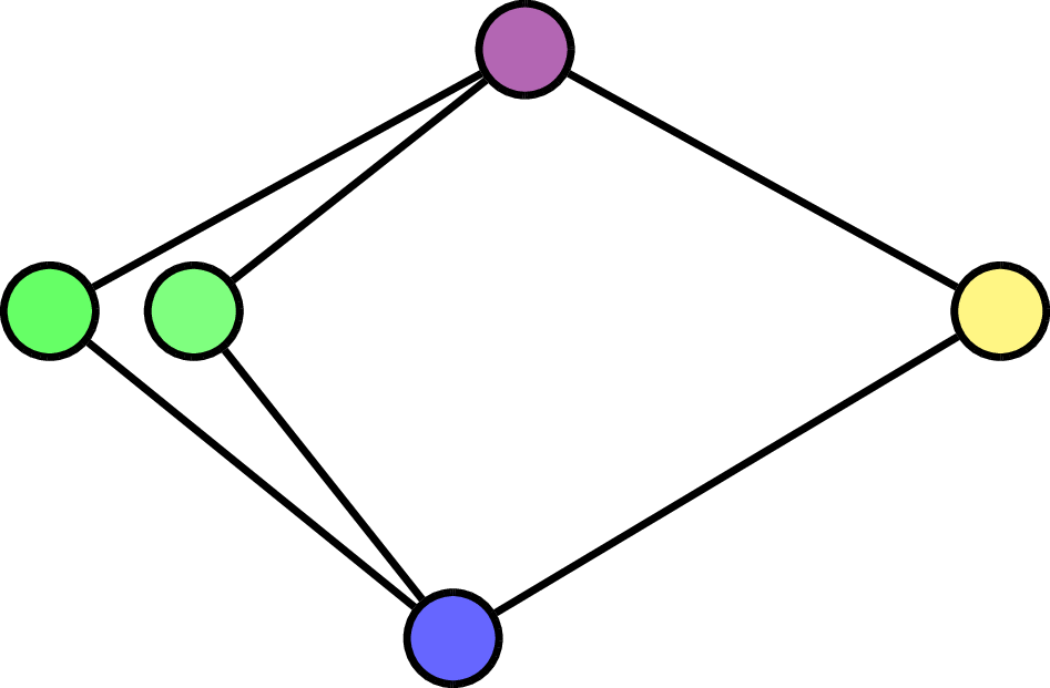
\(F = (\quad\;)\):

\begin{aligned} \pi_F(Y) &= \pi_{[\phantom{m}, \phantom{m}]}(Y) \cdot\pi_{[\phantom{m}, \phantom{m}]}(Y) \\ &= (1+Y)\cdot (1 + 3Y + 2Y^2) \end{aligned}

Self reciprocity

The flag Hilbert–Poincaré series:

Idea: \(\mathsf{fHP}_{\mathcal{A}}\) is equivalent to a multivariate \(p\)-adic integral.

Theorem (M., Voll 2024). For \(\mathcal{A}\) defined over field of characteristic \(0\) and central, then

\mathsf{fHP}_{\mathcal{A}}\left(Y^{-1},(T_x^{-1})_{x\in\mathcal{L}(\mathcal{A})}\right) = (-Y)^{-\mathrm{rk}(\mathcal{A})} T_{\hat{1}} \cdot \mathsf{fHP}_{\mathcal{A}}(Y, \bm{T}).
\mathsf{fHP}_{\mathcal{A}}(Y, \bm{T}) = \displaystyle\sum_{F\in\Delta(\mathcal{L}(\mathcal{A})\setminus \{\hat{0}\})} \pi_F(Y) \prod_{x\in F} \dfrac{T_x}{1 - T_x}

For \(x\in\mathcal{L}(\mathcal{A})\), set

\lambda(x) = \# \left\{ H\in\mathcal{A} ~\middle|~ x\subseteq H \right\}.

All potential poles come from combinatorial data:

\mathrm{Re}(s) \in \left\{ -\dfrac{\mathrm{codim}(x)}{\lambda(x)} ~\middle|~ x\in\mathcal{L}(\mathcal{A})\setminus\{\hat{0}\}\right\} \subseteq \mathbb{Q}\cap [-1,0)

Back to Igusa zeta functions

is the Igusa zeta function associated to \(\mathcal{A}\).

Theorem (M., Voll 2024). If \(\mathcal{A}\) defined over \(\mathbb{Q}\), then for all but finitely many primes \(p\),

\mathsf{fHP}_{\mathcal{A}}\left(-p^{-1}, (p^{-\mathrm{codim}(x) - \lambda(x) s})_{x\in\mathcal{L}(\mathcal{A})}\right)

Example.

\mathcal{\mathsf{B}_3} :~ x_1x_2x_3(x_1^2 - x_2^2)(x_1^2 - x_3^2)(x_2^2 - x_3^2)
\begin{align*} \dfrac{1 - p^{3-s} \cdot \left.Z_{\mathsf{B}_3}(-3-s)\right|_{p\to p^{-1}}}{(1 - p^{3-s})} &= \dfrac{1 + 15p^{-s} - 23p^{1-s} + 7p^{2-s} + \cdots + p^{42-17s}}{(1 - p^{2-s})^2(1 - p^{7-3s})(1 - p^{10 - 4s})(1 - p^{24 - 9s})} \\[1.25em] \end{align*}

Back to our original data:

= 1 + (9p^2 + \cdots)p^{-s} + (22p^4 + \cdots)p^{-2s} + \cdots

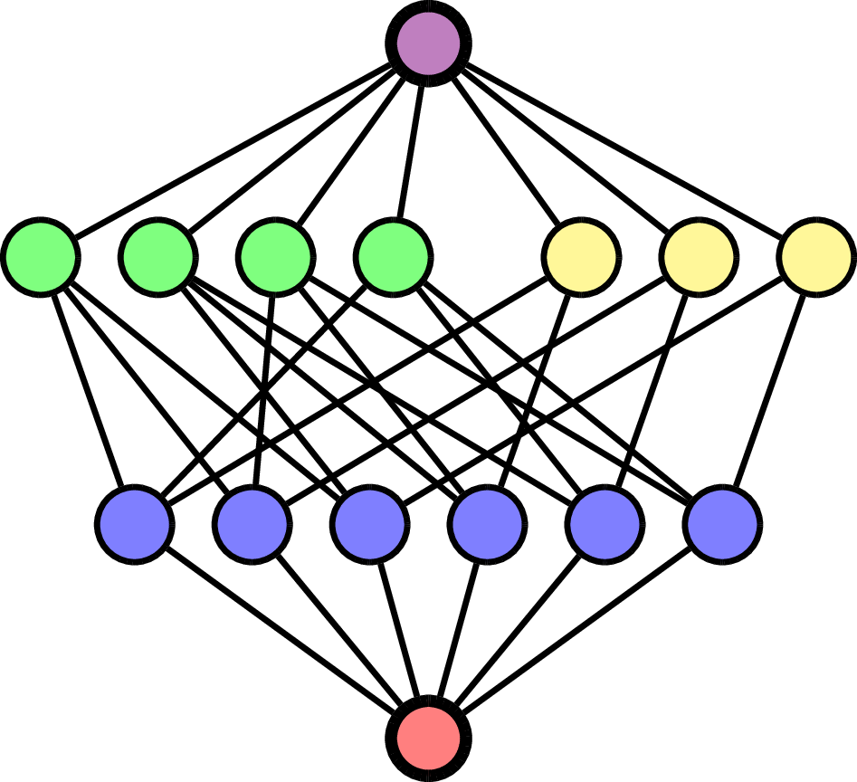
\(\mathcal{L}(\mathsf{B}_3)\)

Z_{\mathsf{B}_3}(s) = \dfrac{(1 - p^{-1})(1 - 8p^{-1} + 15p^{-2} + \cdots + 15p^{-6-9s} - 8p^{-7-9s} + p^{-8-9s})}{(1 - p^{-1-s})(1 - p^{-2-3s})(1 - p^{-2-4s})(1 - p^{-3-9s})}
\lambda(\phantom{m}) = 9
\lambda(\phantom{m}) = 1
\lambda(\phantom{m}) = 2
\lambda(\phantom{m}) = 3
\lambda(\phantom{m}) = 4

A different coarsening

Set each \(T_x=T\) — coarse flag Hilbert–Poincaré series:

Nice form:

\begin{align*} \mathcal{N}_{\mathsf{B}_3}(Y, T) &= 1 + 9Y + 23Y^2 + 15Y^3 + 20T + 76Y T \\ &\quad + 76Y^2T + 20Y^3T + 15T^2 + 23Y T^2 + 9Y^2T^2 + Y^3T^2 \end{align*}
\mathsf{cfHP}_{\mathcal{A}}(Y, T) = \dfrac{\mathcal{N}_{\mathcal{A}}(Y, T)}{(1 - T)^{\mathrm{rk(\mathcal{A})}}}
\mathsf{cfHP}_{\mathcal{A}}(Y, T) = \displaystyle\sum_{F\in\Delta(\mathcal{L}(\mathcal{A})\setminus \{ \hat{0}\})} \pi_F(Y) \left(\dfrac{T}{1 - T}\right)^{\# F}

of \(\mathcal{L}(\mathcal{A})\)

codim of

maximal elt

Corollary. For every hyperplane arrangement \(\mathcal{A}\), the coefficients of \(\mathcal{N}_{\mathcal{A}}(Y, T)\) are non-negative.

\{\text{maximal flags of }\mathcal{L}(\mathcal{A})\} \times \{\text{subsets of }\{1,\dots, \mathrm{rk}(\mathcal{A})\}\}

Theorem (Dorpalen-Barry, M., Stump +2023). The coefficients of \(\mathcal{N}_{\mathcal{A}}(Y, T)\) count

together with two statistics on the pair.

\mathcal{N}_{\mathcal{A}}(Y, T) = \sum_{(M, S)} Y^{\# S} T^{\mathrm{stat}(M, S)}.

Numerator polynomial looks something like:

Summary

  • Combinatorially defined substitution from flag Hilbert–Poincaré series to Igusa zeta function.
  • Self-reciprocity of flag Hilbert–Poincaré series yield palindromicity of coefficients.
  • Coefficients of numerator of coarse flag Hilbert–Poincaré series are non-negative.

flag Hilbert–Poincaré series

Igusa zeta function

combinatorial "coarsening"